Fuel Economy Regression Case Study

Question

What vehicle characteristics are associated with fuel economy, and how well can they predict it? The analysis answers that in two steps, a one-feature baseline and a full model, and then says plainly what a linear model on this data cannot tell you.

Data

The public Auto MPG dataset: 398 vehicles and 9 columns covering model years 1970 to 1982 (notebook output: “398 rows x 9 columns”). It originated in Carnegie Mellon’s StatLib library, is distributed by the UCI Machine Learning Repository, and is mirrored in seaborn-data, which is the copy the download script fetches. The script writes a provenance record with the source URL, retrieval time, byte count, and SHA-256, and warns if the upstream copy changes. No personal data is involved. Cleaning, with reasons written down: six rows missing horsepower are dropped rather than imputed (392 remain), because horsepower is a headline predictor and inventing 1.5 percent of it would manufacture evidence for the relationship under test; and eight misspelled or shortened manufacturer names (for example chevroelt, vokswagen, toyouta, maxda, chevy, vw) are normalized so that 37 apparent makes become the 29 real ones. Sources: repository README, notebook outputs, docs/process-notes.md.

SQL and schema

Not applicable: the dataset is a single CSV and the analysis runs entirely in pandas. The column dictionary lives in the repository’s data/README.md.

Method

Inspect, clean, transform, visualize, correlate, model, diagnose. Correlation first: weight is the strongest single correlate of mpg (r = 0.83, negative), and weight, displacement, horsepower, and cylinders correlate 0.84 to 0.95 with each other, which is the analysis’s main statistical problem. A power-to-weight ratio is derived from two existing columns. A seeded train and test split (random_state=42; 313 training rows, 79 test rows) is followed by two scikit-learn linear models: a weight-only baseline, fit first so the full model has something to beat, and a full model on six numeric features plus origin. Diagnostics are measured rather than eyeballed: the test set is split into terciles by predicted mpg and the error spread and mean error are reported per tercile. The collinear predictors are deliberately kept, and the reasoning is recorded in the process notes. Sources: README, notebook outputs, docs/process-notes.md.

Result

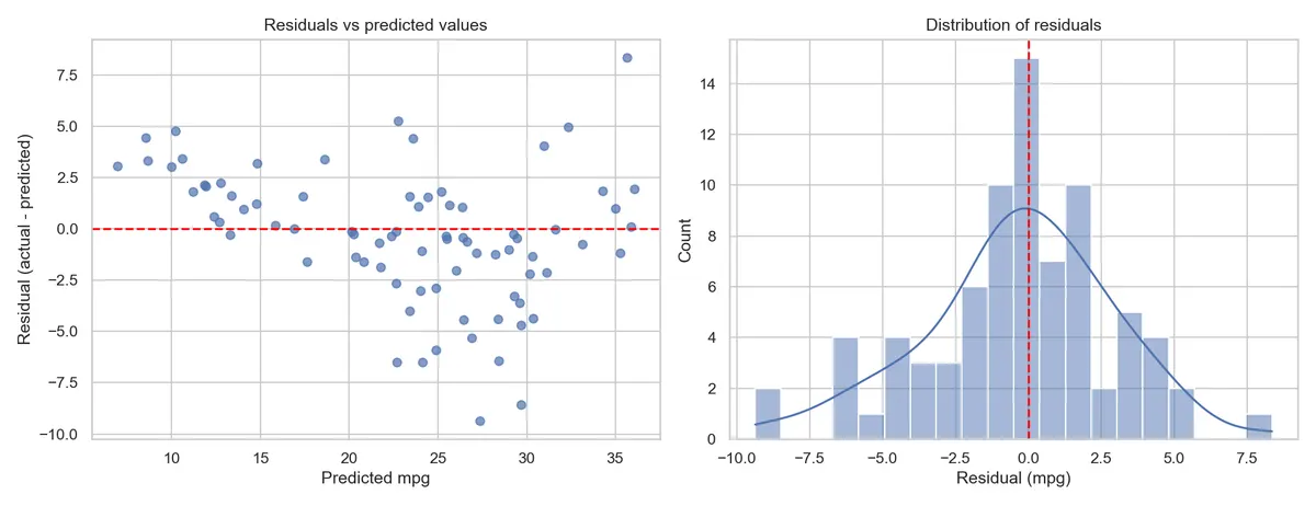
The baseline explains 65.3 percent of the variation in fuel economy on the test set (test R2 0.653); the full model explains 79.2 percent (test R2 0.792), a measured gain of 0.139 with a train to test gap of 0.036, so no meaningful overfitting. The mean residual is 0.35 mpg negative, but the diagnostics show why that number alone would mislead: error spread grows across the terciles (1.81, 2.99, 3.89 mpg) and the mean error flips sign (1.46, negative 1.00, negative 1.46), so the model under-predicts the thirstiest cars and over-predicts the rest. That is the signature of a curved relationship fitted with a straight line, and the near-zero overall residual is two opposite biases cancelling out. Limitations stated in the notebook’s section 17: observational data, so no causal claim; severe collinearity, so coefficients are not interpreted individually; a 1970 to 1982 window that says nothing about modern vehicles; unequal origin groups; six dropped rows; and two violated linear-model assumptions. Sources: README headline table and notebook outputs.

Notebook

notebooks/fuel-economy-analysis.ipynb is committed executed, with every output saved (28 code cells, 27 with outputs), so it reads on GitHub without running anything. Kernel, Restart and Run All reproduces every number above; all randomness is seeded. A clean-room re-run from an empty data folder reproduced every published figure. Rendering the notebook inside this page through Quarto is an open item of the site build (the tool is not yet installed on the build machine); until then the executed notebook on GitHub is the reference.

Repository

github.com/KhaylubThompsonCalvin/fuel-economy-analysis: the notebook, scripts/download_data.py with its provenance record, the column dictionary, six figures exported by the notebook, docs/process-notes.md with the decisions made and rejected, and pinned library versions (Python 3.13.9, pandas 2.3.3, scikit-learn 1.7.2, matplotlib 3.10.6, seaborn 0.13.2, numpy 2.3.5). What I would change next: add a LICENSE file (recommended in the media inventory), and try a transformed target or a nonlinear model to address the curvature the diagnostics found.